The molecules of gas move randomly in any direction. You may think that we have some idea about the molecular speeds of an ideal gas after understanding it's kinetic behaviour where we can find the average of the square of velocity of molecules and we can also find the rms-speed (root-mean-square-speed), however, this is not a complete solution to the distribution of molecular speeds. So, here we define a distribution function which describes the distribution of molecular speeds given by \(f(v)\) called Maxwell-Boltzmann distribution function where \(v\) is the speed of any molecule.
The probability of any molecule having speed between \(v\) and \(v+dv\) is \(f(v)dv\). This is because if \(dN\) is the number of molecules having speed in the interval between \(v\) and \(v+dv\) and \(N\) is the total number of molecules then,
\[\begin{align*} \frac{{dN}}{N} &= f(v)dv \tag{1} \label{1} \\ {\rm{and,}}\quad dN &= Nf(v)dv \tag{2} \label{2} \end{align*}\]
Note that the ratio \(dN/N\) represents the probability. The derivation of Maxwell-Boltzmann distribution function requires statistical approach which we are not going to deal with now but it can be expressed as
\[f(v) = 4\pi {\left( {\frac{m}{{2\pi kT}}} \right)^{3/2}}{v^2}{e^{ - m{v^2}/2kT}} \tag{3} \label{3}\]
In Figure 1 you can see a graph of \(f(v)\) versus \(v\). Note that the Eq. \eqref{1} shows that the function \(f(v)\) is the probability per unit speed interval. At any chosen value of \(v\) on the x-axis, the value of \(f(v)\) represents the distribution of molecular speeds near \(v\) which is proportional to the number of molecules near \(v\). You can see in the graph in Figure 1 that as the temperature increases, more and more molecules move with greater speeds (kinetic energy increases) and the peak of the curve decreases.


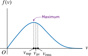
Once you have the expression of Maxwell-Boltzmann distribution function you can find the most probable speed denoted by \(v_\text{mp}\), average speed \(v_\text{av}\) and rms-speed \(v_\text{rms}\). The speed when \(df(v)/dv = 0\) is the most probable speed which is the speed when \(f(v)\) is maximum at the peak of the curve shown in Figure 2. First we denote the constant part in Eq. \eqref{3} by \(c = 4\pi {\left( {m/2\pi kT} \right)^{3/2}}\). To find the most probable speed,
\[\begin{align*} \frac{{df(v)}}{{dv}} &= 0\\ {\rm{or,}}\quad c\frac{{d({v^2}{e^{ - m{v^2}/2kT}})}}{{dv}} &= 0\\ {\rm{or,}}\quad c\left[ {{v^2}\left( {\frac{{ - mv}}{{kT}}} \right){e^{ - m{v^2}/2kT}} + 2v{e^{ - m{v^2}/2kT}}} \right] &= 0\\ {\rm{or,}}\quad c{e^{ - m{v^2}/2kT}}\left[ {2v - \frac{{m{v^3}}}{{kT}}} \right] &= 0 \end{align*}\]
Dividing both sides of the above equation by \(c{e^{ - m{v^2}/2kT}}\) and solving for \(v\) you'll get the most probable speed \(v = v_\text{mp}\):
\[{v_{{\rm{mp}}}} = \sqrt {\frac{{2kT}}{m}} \tag{4} \label{4} \]
You can also find the average speed of molecules. You know that \(dN = Nf(v)dv\). Average speed is the sum of the speeds of all molecules divided by the total number of molecules. To find the average speed we multiply \(dN\) by any speed \(v\) whose integration between limits \(0\) and \(\infty\) is the sum of the speeds of all molecules. Which then divided by the total number of molecules to find the average speed:
\[{v_{{\rm{av}}}} = \int\limits_0^\infty {f(v)v\,dv} \tag{5} \label{5}\]
You can carry out the integration (the hint is use integration by parts method) in above equation and finally the result for the average speed is
\[{v_{{\rm{av}}}} = \sqrt {\frac{{8kT}}{{\pi m}}} \tag{6} \label{6} \]
Another speed you can find is rms-speed (root-mean-square speed) which is the square root of the average of the square of the speed of all molecules. To find the average of the square of \(v\) that is, \({({v^2})_{{\rm{av}}}}\), we replace \(v\) in Eq. \eqref{5} by \(v^2\):
\[{v_{{\rm{rms}}}} = \int\limits_0^\infty {f(v){v^2}\,dv} \tag{7} \label{7}\]
After doing integration in the above equation for the rms-speed, you can finally get the expression for the rms-speed:
\[{v_{{\rm{rms}}}} = \sqrt {\frac{{3kT}}{m}} \tag{8} \label{8}\]
The expression of the rms-speed in the above equation is the same as the expression we obtained from the kinetic theory of an ideal gas.
If you compare Eqs.\eqref{4}, \eqref{6} and \eqref{8} of \(v_\rm{mp}\), \(v_\rm{av}\) and \(v_\rm{rms}\) respectively for any value of \(v\) you will find \(v_\rm{rms} > v_\rm{av} >v_\rm{mp}\) (see Figure 2).


